
ISB-CGC, one of the National Cancer Institute's Cloud Resources, uniquely hosts cancer data including
somatic mutations, copy number variations, gene and, protein expressions, etc. from widely used cancer
datasets including TCGA, TARGET and many more in Google BigQuery.
Google BigQuery is a massively-parallel analytics engine ideal for tabular data. ISB-CGC has combined data scattered over tens of thousands of files into easily accessible BigQuery tables. This novel approach allows our users to quickly analyze data from thousands of patients in ISB-CGC curated BigQuery tables.
- Users can explore and learn more about the ISB-CGC hosted BigQuery tables via an interactive BigQuery Table Search User
Interface. Users can find tables of interest based on category, reference genome build, data type
and free-form text search.
- Users with Google Cloud Platform (GCP) projects can analyze patient, biospecimen, and molecular data from many NCI funded programs such as TCGA, TARGET, CCLE, GTEx all in ISB-CGC's BigQuery tables. SQL queries can be executed in many ways including through the Google Cloud BigQuery web console, Jupyter notebooks, and R scripts.
In this tutorial, you will:
- Analyze gene expression and protein abundance differences between two types of TCGA kidney cancers, Kidney Renal Papillary Carcinoma (TCGA-KIRP) and Kidney Chromophobe (TCGA-KICH).
- Build a cohort of patients with these cancer types and extract their respective gene expression and protein abundance data from ISB-CGC TCGA Google BigQuery tables.
- Connect to Google BigQuery tables from within R for data analysis and visualization
What you'll learn:
- How to explore the ISB-CGC BigQuery Table Search User Interface
- How to build and run queries in the Google BigQuery Console
- How to use R notebooks for data analysis and visualization
- How to use Bioconductor packages on data in ISB-CGC BigQuery tables
A Google Cloud Platform (GCP) Project is required to access and query the data in BigQuery. However, you do not need to enter payment information (i.e. a credit card) to access or query the tables.
To create a new project, follow these steps:
- If you don't already have a Google Account (Gmail or Google Apps), create one.
- Sign-in to Google Cloud Platform console (console.cloud.google.com)
to create a new project.
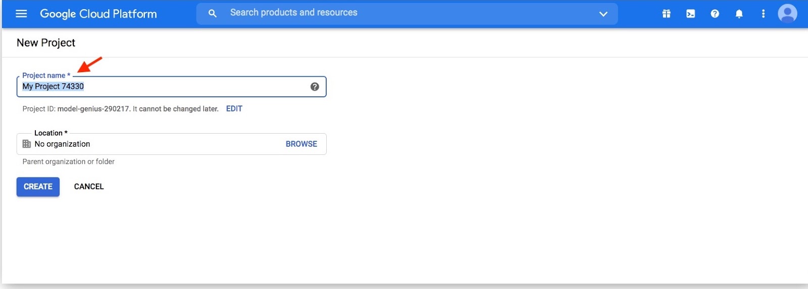
Click on "Select a project" dropdown and click on New Project

Pick a name for your new project then click "Create"
Search for BigQuery in the Google Cloud Platform console

Connect to ISB-CGC's cancer data tables in Google BigQuery
Once on the BigQuery
page, you will see an "Add Data" box with a "Pin a Project" option. Click on "Pin a
Project"

Enter "isb-cgc" then click "pin"

You will now see the isb-cgc open access BigQuery tables on the left-hand side pinned to your project.

No login or special Google Cloud Platform privileges are required to access the ISB-CGC BigQuery Table Search.
Navigate to the ISB-CGC homepage: https://isb-cgc.org and click on the Launch icon in the BigQuery Table Search box.

We want to build a cohort of TCGA patients for which both gene expression and protein abundance data exists.
Let's search for ISB-CGC hosted BigQuery tables that contain information for TCGA gene expression,
protein expression and clinical data.
- Enter TCGA in the Program filter and Clinical Data,
Gene Expression, and Protein Expression in the Data
Type filter.

- To see the table schema of the clinical table, click on the (+) icon.

- Navigate to the Google Cloud Platform (GCP) BigQuery Console by clicking on the "open" button under the table preview or on the "magnifying glass" icon on the right hand side of the Table Search row.

Now that you've found your tables of interest, let's build some queries in the BigQuery console!
On the Google Cloud BigQuery Console we can preview the table, look at the schema (including column names, descriptions, table sizes, etc), and perform queries. The image below shows the preview of the contents of the TCGA Clinical BigQuery table.

Try out these short queries to explore TCGA data by simply entering the SQL commands in the Query Editor and clicking Run:
Identifying how many patients there are with TCGA kidney cancers.
SELECT distinct (case_barcode)
FROM `isb-cgc.TCGA_bioclin_v0.clinical_v1`
WHERE project_short_name LIKE "TCGA-KI%"
Building a cohort based on clinical variables.
SELECT
  distinct(case_barcode)
FROM
  `isb-cgc.TCGA_bioclin_v0.clinical_v1`
WHERE
  project_short_name LIKE "TCGA-KI%"
  AND primary_therapy_outcome_success = 'Complete Remission/Response'
  AND vital_status = 'Alive'
Compute basic statistics such as average and standard deviations.
SELECT
  AVG(age_at_diagnosis) as mean_age_at_dx,
  STDDEV_SAMP(age_at_diagnosis) as stddev_age_at_dx
FROM
  `isb-cgc.TCGA_bioclin_v0.clinical_v1`
WHERE
  project_short_name LIKE "TCGA-KI%"
  AND primary_therapy_outcome_success = 'Complete Remission/Response'
  AND vital_status = 'Alive'
  AND age_at_diagnosis is not NULL
Joining tables to access variant data for our cohort.
SELECT
  clin_table.case_barcode,
  var_table.Hugo_Symbol,
  var_table.Variant_Type,
  var_table.Variant_Classification,
  var_table.SIFT,
  var_table.PolyPhen
FROM
  `isb-cgc.TCGA_bioclin_v0.clinical_v1` as clin_table
JOIN
  `isb-cgc.TCGA_hg38_data_v0.Somatic_Mutation` as var_table
ON
  clin_table.case_barcode = var_table.case_barcode
  AND clin_table.project_short_name = var_table.project_short_name
WHERE
  clin_table.project_short_name LIKE "TCGA-KI%"
  AND clin_table.primary_therapy_outcome_success =
        'Complete Remission/Response'
  AND clin_table.vital_status = 'Alive'
  AND var_table.Hugo_Symbol = 'VHL'
You've built some cool queries here, but now you may want to visualize the query results. Let's generate some plots using R.
It is really simple to access data in BigQuery tables from R through:
- R or RStudio installed locally on your machine
- RStudio Cloud (limited free version great for data exploration)
- R notebook on a virtual machine (VM) within the Google Cloud AI Platform (requires a Google Cloud Platform project with a billing account associated with it)
In this tutorial, we will be running an R instance through RStudio Cloud.
Navigate to the RStudio Cloud webpage: https://rstudio.cloud

Login to RStudio Cloud using your Google ID.

Provide a name for your account

Creating a new Project will deploy an R console
Let's begin working in the R console!

The bigrquery package is designed to work with data stored in Google BigQuery tables. More information about the package can be found here: https://bigrquery.r-dbi.org/
Enter each block of code below into the RStudio Cloud terminal.
Install the required bigrquery package and enter in your newly created Google Cloud Platform project ID
install.packages("bigrquery")
library(bigrquery)
project <- "your project" #Replace with your newly created project name
Let's build the query we made in the Google BigQuery web console here in R.
In R, the query is saved in a variable called "sql" .
The query results are pushed into a temporary BigQuery table which can be downloaded into an R dataframe or matrix.
# Query the clinical table for our cohort.
# Retrieve Age at Diagnosis and Clinical Stage for Kidney Cancer data.
sql <- "Select case_barcode, age_at_diagnosis, project_short_name, clinical_stage
        from `isb-cgc.TCGA_bioclin_v0.Clinical` as clin
         where project_short_name in ('TCGA-KIRP', 'TCGA-KICH')"
options(scipen=20)
clinical_tbl <- bq_project_query (project, query = sql) #Put data in temporary BQ table
clinical_data <- bq_table_download(clinical_tbl) #Put data into a dataframe
head(clinical_data)
The first 5 rows of the clinical_data dataframe looks like this:

Let's analyze the data we just queried from the BigQuery table with some basic R functions.
What's the age distribution of the patients in our cohort of TCGA kidney cancer patients (TCGA-KICH and TCGA-KIRP)?
# Plot two histograms of age of diagnosis data of our cohort.
layout(matrix(1:2, 2, 1))
hist(clinical_data[clinical_data$project_short_name == "TCGA-KIRP",]$age_at_diagnosis,
    xlim=c(15,100), ylim=c(0,40), breaks=seq(15,100,2),
    col="#FFCC66", main='TCGA-KIRP', xlab='Age at diagnosis (years)')

hist(clinical_data[clinical_data$project_short_name == "TCGA-KICH",]$age_at_diagnosis,
    xlim=c(15,100), ylim=c(0,40), breaks=seq(15,100,2),
    col="#99CCFF", main='TCGA-KICH', xlab='Age at diagnosis (years)')
# Create SQL query to retrieve the mean gene expression and mean protein expression per project/case.

# Load it into a dataframe.
sql_expression <-
"With gexp as
(SELECT project_short_name, case_barcode, gene_name, avg(HTSeq__FPKM) as mean_gexp
FROM `isb-cgc.TCGA_hg38_data_v0.RNAseq_Gene_Expression`
WHERE project_short_name in ('TCGA-KIRP', 'TCGA-KICH') AND gene_type = 'protein_coding'
GROUP BY project_short_name, case_barcode, gene_name
),
pexp as
(SELECT project_short_name, case_barcode, gene_name, avg(protein_expression) as mean_pexp
FROM `isb-cgc.TCGA_hg38_data_v0.Protein_Expression`
WHERE project_short_name in ('TCGA-KIRP', 'TCGA-KICH')
GROUP BY project_short_name, case_barcode, gene_name
)
SELECT gexp.project_short_name, gexp.case_barcode, gexp.gene_name, gexp.mean_gexp, pexp.mean_pexp
FROM gexp
inner join pexp
on gexp.project_short_name = pexp.project_short_name AND gexp.case_barcode = pexp.case_barcode AND gexp.gene_name = pexp.gene_name"

#disable scientific notation
options(scipen=20)

expression_data <- bq_table_download(bq_project_query (project, query = sql_expression)) #Put data into a dataframe
head(expression_data)

expression_data$id <- paste(expression_data$project_short_name, expression_data$case_barcode, sep='.')
cases <- unique(expression_data$id)

# Transform the expression_data data frame, so that columns are samples, rows are genes.
list_exp <- lapply(cases, function(case){
    temp <- expression_data[expression_data$id == case, c('gene_name', 'mean_gexp')]
    names(temp) <- c('gene_name', case)
    return(temp)
})

gene_exps <- Reduce(function(x, y) merge(x, y, all=T, by="gene_name"), list_exp)
head(gene_exps)
dim(gene_exps)
# Perform the same transform for protein abundance.
  list_abun <- lapply(cases, function(case){
      temp <- expression_data[expression_data$id == case, c('gene_name', 'mean_pexp')]
      names(temp) <- c('gene_name', case)
      return(temp)
  })
  pep_abun <- Reduce(function(x, y) merge(x, y, all=T, by="gene_name"), list_abun)
  head(pep_abun)
  dim(pep_abun)
# Separate the cohorts (types of kidney cancer) into two dataframes and
# generate a scatterplot of gene expression and protein abundance.
# Gene expression first.
exp_p <- gene_exps[,grep('KIRP', names(gene_exps))]
exp_c <- gene_exps[,grep('KICH', names(gene_exps))]
plot(log(rowMeans(exp_p)), log(rowMeans(exp_c)),
    xlab='log(FPKM KIRP)', ylab='log(FPKM KICH)',
    xlim=c(-3.5,7.5), ylim=c(-3.5,7.5), pch=19, cex=2,
    col=rgb(178,34,34,max=255,alpha=150))
Let's compare the protein expression between KIRP and KICH.
# Get Protein expression second
abun_p <- pep_abun[,grep('KIRP', names(pep_abun))]
abun_c <- pep_abun[,grep('KICH', names(pep_abun))]
plot(rowMeans(abun_p), rowMeans(abun_c),
   xlab='KIRP protein abundance', ylab="KICH protein abundance",
   xlim=c(-0.25,0.3), ylim=c(-0.25,0.3), pch=19, cex=2,
   col=rgb(140,140,230,max=255,alpha=150))
We've shown you how to access and analyze data in BigQuery using base functions in R. There are a number of bioconductor packages designed for TCGA data. How can you use them with data in ISB-CGC BigQuery tables?
We demonstrate how to use the Bioconductor package MAFtools, which has capabilities to summarize, analyze and visualize Mutation Annotation Format (MAF) data on TCGA somatic mutation data stored in BigQuery tables.
Let's first install and load the MAFtools package.
#Load bioconductor package to analyze and visualize Mutation Annotation Format (MAF) data.
if (!requireNamespace("BiocManager", quietly = TRUE))
    install.packages("BiocManager")
BiocManager::install("maftools")
library("maftools")
MAFtools requires MAF files as input that are read in by the read.maf function. This function reads in the MAF files, summarizes the information and stores them as a MAF object. Our objective is to turn data from the ISB-CGC TCGA MAF BigQuery table into a MAF object.
Let's build a query of our cohort of kidney cancer patients (TCGA-KICH and TCGA-KIRP) from our somatic mutation BigQuery table. MAFtools requires MAF input files to consist of columns with the fields that we're selecting for in the queries below.
# Use BigQuery to load TCGA somatic mutation data for our cancers of interest.
sql_kich<-"SELECT Hugo_Symbol, Chromosome, Start_Position, End_Position, Reference_Allele, Tumor_Seq_Allele2, Variant_Classification, Variant_Type, sample_barcode_tumor  FROM
`isb-cgc.TCGA_hg38_data_v0.Somatic_Mutation` WHERE project_short_name = 'TCGA-KICH'"

sql_kirp<-"SELECT Hugo_Symbol, Chromosome, Start_Position, End_Position, Reference_Allele, Tumor_Seq_Allele2, Variant_Classification, Variant_Type, sample_barcode_tumor FROM
`isb-cgc.TCGA_hg38_data_v0.Somatic_Mutation` WHERE project_short_name = 'TCGA-KIRP'"

#Put data into a dataframe
maf_kich <- bq_table_download(bq_project_query (project, query = sql_kich))
maf_kirp <- bq_table_download(bq_project_query (project, query = sql_kirp))

#Rename column 9 to the field name required by maftools.
colnames(maf_kich)[9] <- "Tumor_Sample_Barcode"
colnames(maf_kirp)[9] <- "Tumor_Sample_Barcode"

head(maf_kich)
head(maf_kirp)
We now have our cohort MAF information from our query saved in dataframes. Let's convert them into MAF objects.
# Convert data frames to maftools objects.
kich <- read.maf(maf_kich)
kirp <- read.maf(maf_kirp)
Once in MAF object format, we can now use the MAFtools built-in plot functionality on the data we have queried from the BigQuery somatic mutation table.
#Maftools plots
plotmafSummary(maf = kich, rmOutlier = TRUE, addStat = 'median', dashboard = TRUE, titvRaw = FALSE)
plotmafSummary(maf = kirp, rmOutlier = TRUE, addStat = 'median', dashboard = TRUE, titvRaw = FALSE)
Congratulations, you've queried cancer data on the cloud using BigQuery!
What's next?
- Learn more about what ISB-CGC has to offer at our homepage and documentation page
- Requesting Cloud Credits
- General Jupyter Notebooks
- Statistical Notebooks
- Pipelines
- Google Cloud AI Platform for R or Python Notebooks
- SQL syntax examples
- Explore ISB-CGC BigQuery tables
- Publishing or presenting results derived from using our platform? Don't forget to cite us!
Reynolds, S. M. et al. The ISB Cancer Genomics Cloud: a flexible cloud-based platform for cancer genomics
research. Cancer Res. 77, e7–e10 (2017).
ISB-CGC is a component of the NCI Cancer Research Data Commonsopens a new tab and has been funded in whole or in part with Federal funds from the National Cancer Institute, National Institutes of Health, Department of Health and Human Services, under Contract No. HHSN261201400008C and ID/IQ Agreement No. 17X146 under Contract No. HHSN261201500003I.